VL-JEPA: What Changes When a Model Predicts Answer Embeddings?
If a language model already computes continuous hidden vectors, what changes when VL-JEPA predicts an embedding? The useful distinction is the prediction target, the training objective, and which outputs require text generation. You cannot identify the difference simply by asking whether the model contains a latent space.
VL-JEPA learns to predict a representation of an answer from visual input and a query. You can compare that prediction with candidate answer embeddings, retrieve matching videos, or pass it to a separate text decoder. This separation matters when you need frequent visual updates but only occasional written descriptions.
The paper was first submitted in December 2025 and revised in February 2026. This explanation uses version 2, including its distinction between the main model and the controlled experiment used to measure parameter savings.
A hidden state is not the same thing as a supervised target
In a standard autoregressive transformer, a hidden vector h_t is projected to vocabulary logits. A softmax turns those scores into probabilities for the next token. Training rewards the model for assigning probability to the observed target token; generation repeats this process while conditioning on earlier tokens. The original Transformer paper, section 3.4, describes this output projection and softmax.
Those hidden states can contain semantic information. Continuous representations and token prediction are compatible. Also, the hidden vector before vocabulary projection differs from the logits immediately before softmax: the latter already have one coordinate per vocabulary item. Calling both “pre-softmax latents” hides a useful architectural distinction.
VL-JEPA changes what the predictor must match. Its target is the output of a text encoder applied to the answer, rather than the next token in that answer. In the main implementation, predictor outputs are pooled and projected into the same 1,536-dimensional space as the encoded target. The predictor uses bidirectional attention over visual and query embeddings, rather than generating answer tokens sequentially. VL-JEPA, sections 2–3.1.
For an illustrative example, consider “a person opens the door” and “someone pulls the door open.” An answer encoder may place these descriptions close together. Predicting their shared information could be easier than modeling each wording separately. But this is an intended property of the representation, not a guarantee that every paraphrase maps nearby or that every important difference survives compression.
The same caution applies to “the door opens” and “the door closes.” You want those answers separated even though most words overlap. VL-JEPA evaluates sensitivity to changed objects, attributes and relations in its text-encoder experiments. Its scores remain imperfect. A predicted vector is not automatically a calibrated region of possible answers or a probability distribution over meanings.
What the model actually trains
The main architecture has four components: a vision encoder, a query-conditioned predictor, an answer encoder, and an optional answer decoder. The main implementation freezes its V-JEPA 2 vision encoder while jointly training the predictor and answer encoder. The decoder is outside the main embedding-prediction training phase. Architecture and training details.
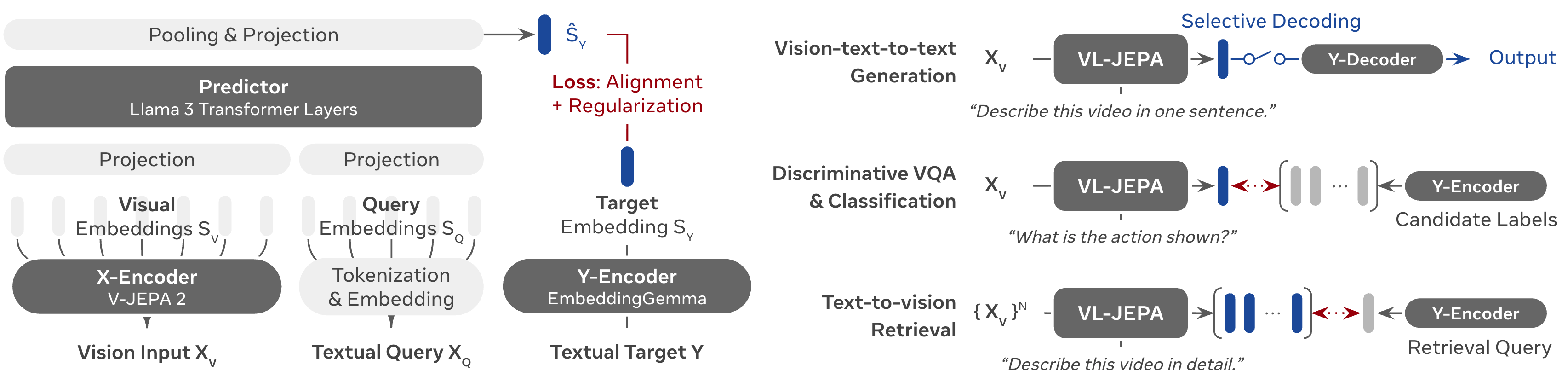 Figure 1. The paper's architecture separates embedding prediction from text readout. “Alignment + regularization” is implemented with bidirectional InfoNCE in this study. Source: Chen et al., VL-JEPA, Figure 2, CC BY 4.0.
The objective is bidirectional InfoNCE. It pulls corresponding predicted and target embeddings together while distinguishing them from other examples in the batch. This contrastive structure helps prevent representation collapse, in which every input receives the same uninformative vector. The paper explicitly leaves VICReg and SIGReg for future investigation; neither is the objective used for the reported VL-JEPA model. Training objective.
InfoNCE can itself be expressed using normalized scores over batch examples. Thus “JEPA removes softmax” is not an adequate explanation. The important change is from predicting vocabulary items at successive answer positions to supervising a complete answer representation. Query tokenization remains, and text generation still needs a decoder when the application requests words.
You can trace an illustrative question, “What is the person doing?”, through three uses of the same prediction:
| Requested output | What happens after embedding prediction |
|---|---|
| Choose an action label | Encode candidate labels and select the closest one. |
| Retrieve a matching video | Compare the query embedding with predicted embeddings of candidate videos. |
| Write a description | Send the predicted embedding to the text decoder. |
These are the inference paths described in section 2. The reported VQA evaluation uses candidate-answer selection. Its results therefore should not be read as a demonstration of unrestricted conversational generation. VQA protocol.
How this differs from latent diffusion
Latent diffusion also works with continuous representations, so the presence of a latent space does not distinguish the methods. You need to inspect what produces the latent, what loss shapes it, and what the system must reconstruct.
The original latent diffusion model uses an autoencoder to compress an image into a spatial feature grid and reconstruct an image from it. Perceptual and adversarial losses encourage useful reconstructions; this is more than a simple pixel-error compressor. A diffusion model then learns generation in that latent space. Rombach et al., sections 3.1–3.2.
The original DiT applies a transformer to patches of a noised VAE latent grid, predicts diffusion quantities, and ultimately uses the VAE decoder to produce an image. “Transformer” describes the denoising architecture; it does not make its training target equivalent to VL-JEPA's answer embedding. Peebles and Xie, sections 3–4.
| Property | VL-JEPA | Original latent diffusion / DiT |
|---|---|---|
| Target representation | Encoded textual answer | Spatial image latent |
| Prediction training | Contrastive answer-embedding alignment | Denoising objective in image-latent space |
| Decoder's role | Read out text when requested | Recover an image from a sampled latent |
| Output fidelity requirement | Useful answer semantics for the evaluated task | Sufficient visual information for image synthesis |
This comparison concerns these implementations, not every possible JEPA or diffusion system. Reconstruction-oriented latents can contain semantic information, and perceptual compression deliberately discards some details. Conversely, VL-JEPA's representations do not come with a guarantee of pure semantics. The defensible distinction is their objectives and required outputs, rather than a binary split between “pixels” and “meaning.”
What selective decoding saves
Imagine you are monitoring a video of someone stirring a bowl. Most consecutive frames may warrant the same description; a transition to pouring the contents might warrant a new one. This is an illustrative use case for deciding when to decode a changing embedding stream. It is not a rule that simple questions need fewer answer embeddings than complex questions.
In the paper's experiment, temporally constrained clustering groups predicted embeddings into coherent segments. The method selects segment midpoints and decodes either the corresponding embedding or a pooled segment embedding. Evaluation uses EgoExo4D validation videos and matches each annotation to its nearest decoded output in time. Selective-decoding protocol.
| Reported comparison | Interpretation |
|---|---|
| Uniform decoding at 1 Hz | One text-decoding operation per second. |
| Selective decoding at 0.35 Hz | Similar caption quality with fewer selected decoding points. |
| Approximately 2.85× reduction | Ratio of decoding frequencies, not a measured universal latency multiplier. |
The quality measure is CIDEr, a caption-overlap metric applied to the temporally matched descriptions. This experiment does not establish identical performance on all tasks. Nor does segment clustering by itself establish the latency of a causal, live deployment: an online system must specify how much future context its event detector uses. The paper separately describes possible online monitoring through smoothing and change detection. Sections 2 and 4.6.
The controlled captioning experiment reports comparable latency when both systems actually generate text. The advantage comes from being able to skip text generation for some outputs. This is different from speculative decoding, which accelerates token generation using a draft-and-verification procedure. VL-JEPA, section 4.5; Leviathan et al..
Parameter savings and downstream fine-tuning
The headline “50% fewer trainable parameters” comes from a specific controlled experiment. It compares a roughly 0.5B predictor with a 1B autoregressive language model using a matched visual encoder and training setup. This is separate from the main model reported as 1.6B parameters. It does not mean every deployment or downstream fine-tuning run uses half the memory or half the compute. Controlled comparison.
The main model has caption-based pretraining followed by supervised fine-tuning for question answering and other tasks. Its supervised mixture includes in-domain examples, so the authors distinguish the base model's zero-shot evaluation from the fine-tuned model's results. The visual encoder remains frozen in the described setup. Training stages.
For a downstream comparison, you should specify which components are trainable, whether the target encoder changes, and whether the output requires a decoder. Count frozen and trainable parameters separately; then measure quality, peak memory, training time and inference latency on the actual task. These are evaluation recommendations, not savings established by the paper.
The results also show why you should evaluate more than the task used for adaptation. The fine-tuned model improves classification after exposure to in-domain data, but its text-encoder scores on SugarCrepe++ and VISLA are lower than those of the base model. The paper does not establish that fine-tuning uniformly improves representation quality. Classification results; text-encoder evaluation.
When the distinction is useful
VL-JEPA gives you an answer representation that can be used before deciding to generate text. Its contribution is an evaluated way to separate those operations, with promising results under the paper's specific training and inference protocols. It does not establish that token-based models lack semantics or that embedding prediction is universally better.
Before applying VL-JEPA, write down the output your application needs: a ranking, a label, a changing event description, or exact prose. Then test the corresponding inference path and count how often it really needs text decoding. That exercise makes the paper's efficiency claims much easier to assess. For another example of separating a model output from the conclusion it supports, see A FASTA file is not a specification.
Revision note, 23 September 2026: corrected the training objective, pre-softmax comparison, diffusion comparison, selective-decoding interpretation and parameter-count framing; added downstream fine-tuning limitations. Removed unsupported claims about human cognition and unrelated world-model capabilities.
Help improve this article
Found an error or a better source? Leave a note here, or highlight a passage to comment on it.